Creating Accessible Spreadsheets in Microsoft Excel 2010/13 (Windows) & 2011 (Mac)

Screen readers and Excel

Users who are blind rely on software called a screen reader to interact with spreadsheets.

• Screen readers will read the cell number as users navigate from cell to cell (e.g., “Grand Total A 23").
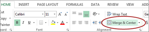
• Spanned cells will be identified by a screen reader (e.g., “Budget A1 through G1”). If content spans multiple cells visually, these cells should be merged. To merge cells, select Home and the Merge menu.
  Merged cells should not be used in tables. They can be confusing for screen reader users who expect one row and/or column header for each cell.
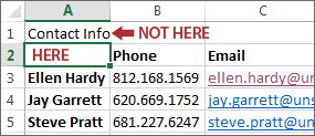
• A screen reader user will usually start with the first cell (A1), so this is a good place to put important information about the sheet.
• Be careful with empty rows and columns. While they may sometimes be necessary to visually separate data, they can cause a screen reader user to think the sheet has ended, even when it has not.

Images and Charts

• While images can be given alternative text in the same way as other Office tools (see other cheatsheets), they can sometimes introduce reading order issues and should typically not be added to spreadsheets.
• Charts cannot be given alternative text. Ensure the data used to create the chart is available and clearly structured, and preferably precedes the chart.

Other principles

• Spell check is not automatic as it is in Word/PowerPoint. Make sure to spell check each sheet.
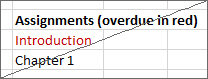
• Do not use color alone to convey information.
Inaccessible       Accessible

Table ‘Headers’

If your spreadsheet includes tables, there is a special way to add table ‘header’ information that will be read in some screen readers. Tables can be identified with formula names of Title, TitleRegion, and others.

• These formulas do not update when the table changes, so be sure your table is complete first.
• This only works for a single level of headers. Complex tables will need to be simplified or restructured.

One table per sheet:

For sheets with one table only, select the cell in the upper-left corner of the table (not the table title).

In Windows, select Formulas> Define Name and the New Name dialog opens. In Mac, select Insert> Name> Define and the Define Name dialog opens.

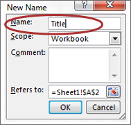
In the Name field, replace the existing text with one of the following 3 values, depending on your table layout:

• If the table has column and row headers, enter Title
• If the table has row headers only, enter RowTitle
• If the table has column headers only, enter ColumnTitle

Don't Confuse "Column" and "Row" headers. Remember that ColumnTitle is for vertical headers and RowTitle is for horizontal headers. Also be sure to type RowTitle or ColumnTitle as one word, without a space.

After entering the correct value in the Name field, select Ok. Although the initial text is still visible, accessibility information has been added for a screen reader user.

Only add a Name to the first cell in the table. Do not repeat this step for other header cells within the same table.

Multiple tables per sheet:

If a single sheet has multiple tables, if the table has sortable columns, or if you want to specify an explicit beginning and end of a table, you need to use TitleRegion.

Select the cell in the upper-left corner of the table (not the table title). In Windows, select Formulas> Define Name and the New Name dialog opens. In Mac, select Insert> Name> Define and the Define Name dialog opens.

In the Name field, enter TitleRegion followed by the following 4 values (no spaces, separated by periods):

1. Unique number within the sheet (e.g., 1 for the first table)
2. First (upper-left) cell in the table (e.g., A2)
3. Last (lower-right) cell in the table (e.g., C5)
4. Sheet number (e.g., 2 for the second tab in the workbook)

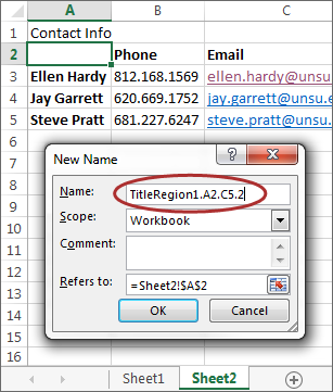
The above table Name would be TitleRegion1.A2.C5.2

Note: RowTitleRegion or ColumnTitleRegion can be used for tables that only have row or column headers.

After entering the correct value in the Name field, select Ok. This table is now accessible. Repeat this process for every table on the sheet, remembering to select the upper-left corner cell of each new table.

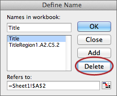
Deleting formula names

You may occasionally create a formula name for the wrong field or give a single cell more than one name. These unnecessary formula names should be removed.

1. To remove formula names in Windows, select Formulas> Name Manager. In Mac select Insert> Name> Define.

2. Then choose the desired name and select Delete.